Consensus clustering with modularity maximization

This example demonstrates how to generate “consensus” clustering assignments (Bassett et al., 2013) from potentially disparate clustering solutions. This is particularly useful when the clustering algorithm used is stochastic / greedy and returns different results when run on the same dataset multiple times (e.g., Louvain modularity maximization).

First let’s grab some data to work with. We’re going to download one session of parcellated functional MRI data from the MyConnectome dataset (Laumann et al., 2015). We’ll pick session 73 (though any session would do):

from urllib.request import urlopen
import numpy as np

url = 'https://s3.amazonaws.com/openneuro/ds000031/ds000031_R1.0.2/' \
      'uncompressed/derivatives/sub-01/ses-073/' \
      'sub-01_ses-073_task-rest_run-001_parcel-timeseries.txt'
data = np.loadtxt(urlopen(url).readlines())
print(data.shape)

(518, 630)

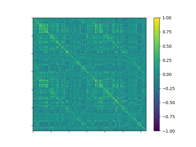
The data has 518 timepoints for each of 630 regions of interest (ROIs) defined by the original authors. We’ll use this to construct an ROI x ROI correlation matrix and then plot it:

import matplotlib.pyplot as plt

corr = np.corrcoef(data.T)

fig, ax = plt.subplots(1, 1)
coll = ax.imshow(corr, vmin=-1, vmax=1, cmap='viridis')
ax.set(xticklabels=[], yticklabels=[])
fig.colorbar(coll)

<matplotlib.colorbar.Colorbar object at 0x7f08693f0200>

We can see some structure in the data, but we want to define communities or networks (groups of ROIs that are more correlated with one another than ROIs in other groups). To do that we’ll use the Louvain algorithm from the bctpy toolbox.

Unfortunately the defaults for the Louvain algorithm cannot handle negative data, so we will make a copy of our correlation matrix and zero out all the negative correlations:

import bct

nonegative = corr.copy()
nonegative[corr < 0] = 0

ci, Q = bct.community_louvain(nonegative, gamma=1.5)
num_ci = len(np.unique(ci))
print('{} clusters detected with a modularity of {:.2f}.'.format(num_ci, Q))

8 clusters detected with a modularity of 0.25.

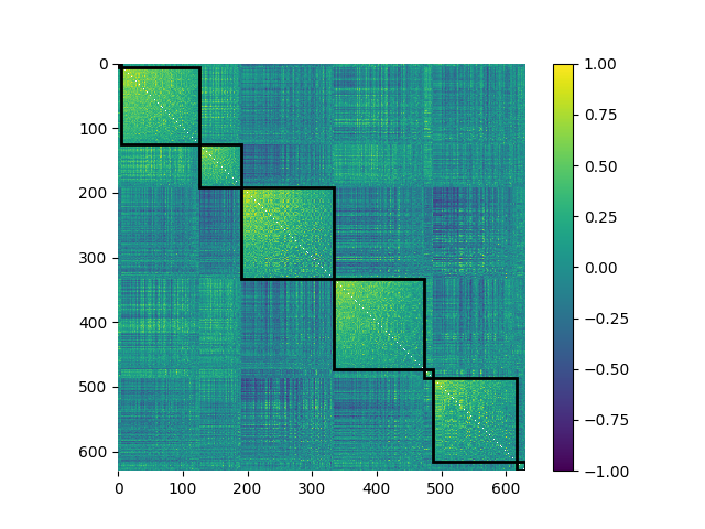
We’ll take a peek at how the correlation matrix looks when sorted by these communities. We can use the plot_mod_heatmap() function, which is a wrapper around plt.imshow(), to do this easily:

from netneurotools import plotting

plotting.plot_mod_heatmap(corr, ci, vmin=-1, vmax=1, cmap='viridis')

<Axes: >

The Louvain algorithm is greedy so different instantiations will return different community assignments. We can run the algorithm ~100 times to see this discrepancy:

ci = [bct.community_louvain(nonegative, gamma=1.5)[0] for n in range(100)]

fig, ax = plt.subplots(1, 1, figsize=(6.4, 2))
ax.imshow(ci, cmap='Set1')
ax.set(ylabel='Assignments', xlabel='ROIs', xticklabels=[], yticklabels=[])

[Text(64.72222222222221, 0.5, 'Assignments'), Text(0.5, 44.357142857142854, 'ROIs'), [Text(-100.0, 0, ''), Text(0.0, 0, ''), Text(100.0, 0, ''), Text(200.0, 0, ''), Text(300.0, 0, ''), Text(400.0, 0, ''), Text(500.0, 0, ''), Text(600.0, 0, ''), Text(700.0, 0, '')], [Text(0, -50.0, ''), Text(0, 0.0, ''), Text(0, 50.0, ''), Text(0, 100.0, ''), Text(0, 60.0, ''), Text(0, 80.0, ''), Text(0, 100.0, '')]]

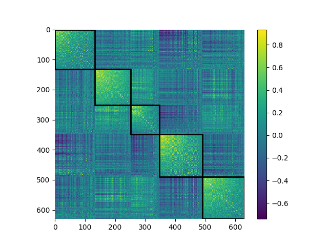
We’ll provide these different assignments to our consensus-finding algorithm which will generate one final community assignment vector:

from netneurotools import modularity

consensus = modularity.find_consensus(np.column_stack(ci), seed=1234)
plotting.plot_mod_heatmap(corr, consensus, cmap='viridis')

<Axes: >

The netneurotools.modularity.consensus_modularity() function provides a wrapper for this process of generating multiple community assignmenta via the Louvain algorithm and finding a consensus. It also generates and returns some metrics for assessing the quality of the community assignments.

Nevertheless, the find_consensus() function is useful for generating a consensus clustering solution from the results of _any_ clustering algorithm (not just Louvain).