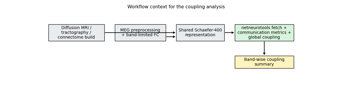
Is structure-function coupling consistent across functional modalities?

This example demonstrates how structural connectivity constrains electrophysiological functional organization. The coupling workflow follows Liu et al. (2023), while the MEG connectome input data are from Shafiei et al. (2022). We derive communication matrices from a consensus structural connectome and compute global structure-function coupling and dominance profiles across haemodynamic and MEG functional connectivity.

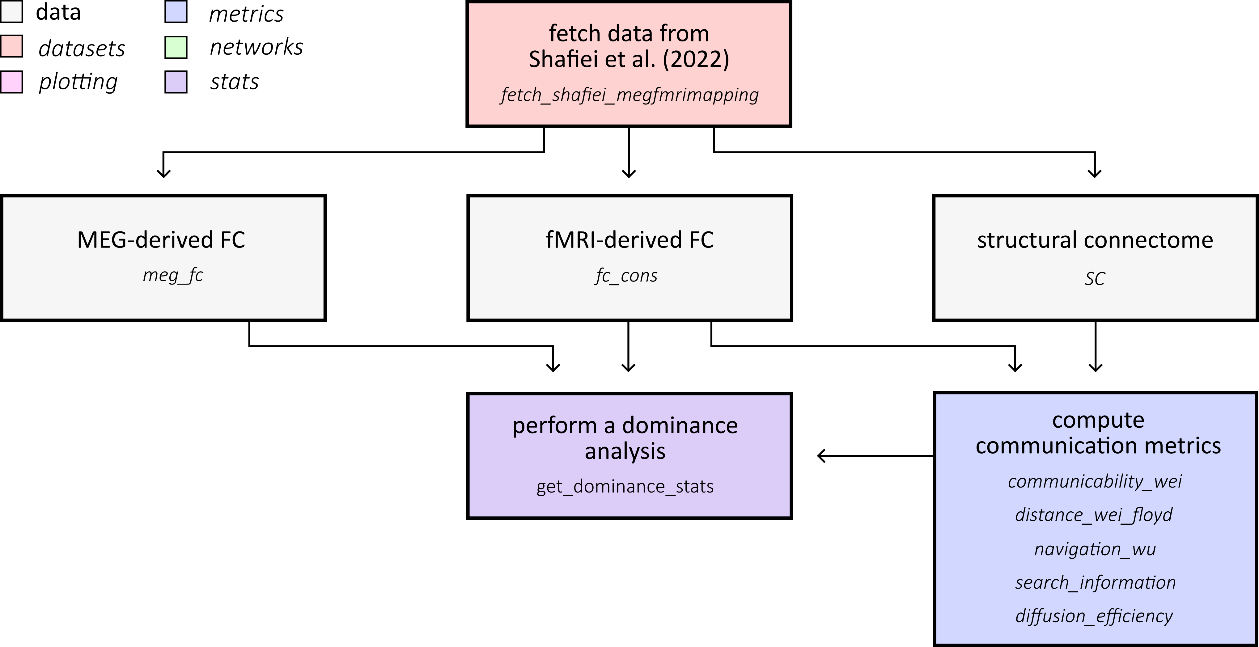
First, fetch the MEG-fMRI mapping dataset from Shafiei et al. (2022).

In this example, we use those data with the structure-function coupling framework from Liu et al. (2023). The dataset contains group-average MEG functional connectivity across six canonical frequency bands and a consensus structural connectome, both parcellated to the Schaefer-400 atlas.

from pathlib import Path

import matplotlib.pyplot as plt
import numpy as np
from matplotlib.colors import ListedColormap, to_rgb
from scipy.spatial.distance import cdist as scipy_cdist

from netneurotools.datasets import fetch_shafiei_megfmrimapping

dataset_root = Path(fetch_shafiei_megfmrimapping())

# MEG FC: shape (n_bands, n_parcels, n_parcels)
megdata = np.load(dataset_root / "data" / "groupFCmeg_aec_orth_schaefer400.npy.npz")
meg_fc = megdata["megfc"]   # (6, 400, 400)
meg_bands = list(megdata["bands"])

# Haemodynamic FC used for the global coupling baseline
fc_cons = np.load(dataset_root / "data" / "groupFCmri_schaefer400.npy")

# Structural connectome
SC = np.load(dataset_root / "data" / "consensusSC_wei_Schaefer400.npy")

print(f"MEG FC shape: {meg_fc.shape} — bands: {meg_bands}")
print(f"fMRI FC shape: {fc_cons.shape}")
print(f"SC shape: {SC.shape}")

Please cite the following papers if you are using this function:
  [primary]:
    Golia Shafiei, Sylvain Baillet, and Bratislav Misic. Human electromagnetic and haemodynamic networks systematically converge in unimodal cortex and diverge in transmodal cortex. PLoS biology, 20(8):e3001735, 2022.
[fetch_single_file] Downloading data from
https://github.com/netneurolab/shafiei_megfmrimapping/archive/ba33fe8f3313f582d9
422edf93d8f1f13309f8e1.tar.gz ...
[fetch_single_file] Downloaded 12328960 of ? bytes.
[fetch_single_file] Downloaded 18358272 of ? bytes.
[fetch_single_file] Downloaded 25427968 of ? bytes.
[fetch_single_file] Downloaded 46669824 of ? bytes.
[fetch_single_file]  ...done. (5 seconds, 0 min)

Downloaded ds-shafiei_megfmrimapping to /home/runner/nnt-data
MEG FC shape: (6, 400, 400) — bands: [np.str_('delta'), np.str_('theta'), np.str_('alpha'), np.str_('beta'), np.str_('lgamma'), np.str_('hgamma')]
fMRI FC shape: (400, 400)
SC shape: (400, 400)

Before computing communication matrices, it helps to make the workflow boundary explicit. The structural connectome and MEG connectivity estimates come from upstream tractography and MEG preprocessing pipelines. In this example, netneurotools enters at the point where harmonized matrices are available in a common parcellation and the question becomes how to transform SC into communication predictors and summarize coupling.

fig, ax = plt.subplots(figsize=(11.5, 3.0))
ax.axis("off")

boxes = [
    (
        0.02,
        0.56,
        0.21,
        0.24,
        "Diffusion MRI /\ntractography /\nconnectome build",
        "#e9ecef",
    ),
    (
        0.27,
        0.56,
        0.19,
        0.24,
        "MEG preprocessing\n+ band-limited FC",
        "#e9ecef",
    ),
    (
        0.50,
        0.56,
        0.18,
        0.24,
        "Shared Schaefer-400\nrepresentation",
        "#e9ecef",
    ),
    (
        0.72,
        0.56,
        0.22,
        0.24,
        "netneurotools fetch +\ncommunication metrics +\nglobal coupling",
        "#d8f3dc",
    ),
    (
        0.72,
        0.16,
        0.22,
        0.18,
        "Band-wise coupling\nsummary",
        "#fff3bf"
    ),
]

for x0, y0, width, height, label, facecolor in boxes:
    rect = plt.Rectangle((x0, y0), width, height, facecolor=facecolor,
                         edgecolor="black", linewidth=1.0)
    ax.add_patch(rect)
    ax.text(x0 + width / 2, y0 + height / 2, label,
            ha="center", va="center", fontsize=10)

arrowprops = dict(arrowstyle="->", lw=1.5, color="black")
ax.annotate("", xy=(0.50, 0.68), xytext=(0.23, 0.68), arrowprops=arrowprops)
ax.annotate("", xy=(0.50, 0.62), xytext=(0.46, 0.62), arrowprops=arrowprops)
ax.annotate("", xy=(0.72, 0.68), xytext=(0.68, 0.68), arrowprops=arrowprops)
ax.annotate("", xy=(0.83, 0.34), xytext=(0.83, 0.56), arrowprops=arrowprops)

ax.set_title("Workflow context for the coupling analysis", fontsize=11)

Text(0.5, 1.0, 'Workflow context for the coupling analysis')

Visualize the MEG connectivity matrices across all six frequency bands. Each band reflects a distinct timescale of neural oscillatory synchrony.

band_colors = ["#4793c1", "#8ab6cf", "#f5c06a", "#ea945a", "#d65f54", "#9b3f7c"]

fig, axes = plt.subplots(2, 3, figsize=(10, 7), constrained_layout=True)
axes = axes.ravel()

for i, (band, color) in enumerate(zip(meg_bands, band_colors)):
    ax = axes[i]
    A = meg_fc[i].copy()
    np.fill_diagonal(A, np.nan)
    ax.imshow(A, cmap="Oranges",
              vmin=np.nanpercentile(A, 5),
              vmax=np.nanpercentile(A, 95))
    ax.set_title(band, fontsize=11, color=color)
    ax.set_xticks([])
    ax.set_yticks([])

Visualize the structural connectivity matrix. Note the characteristic block structure reflecting the spatial organization of cortical regions.

fig, ax = plt.subplots(figsize=(5, 5))
SC_plot = SC.copy()
np.fill_diagonal(SC_plot, np.nan)
ax.imshow(SC_plot, cmap="Greys",
          vmin=np.nanpercentile(SC_plot[SC_plot > 0], 5),
          vmax=np.nanpercentile(SC_plot[SC_plot > 0], 95))
ax.set_title("Structural Connectivity", fontsize=12)
ax.set_xticks([])
ax.set_yticks([])

[]

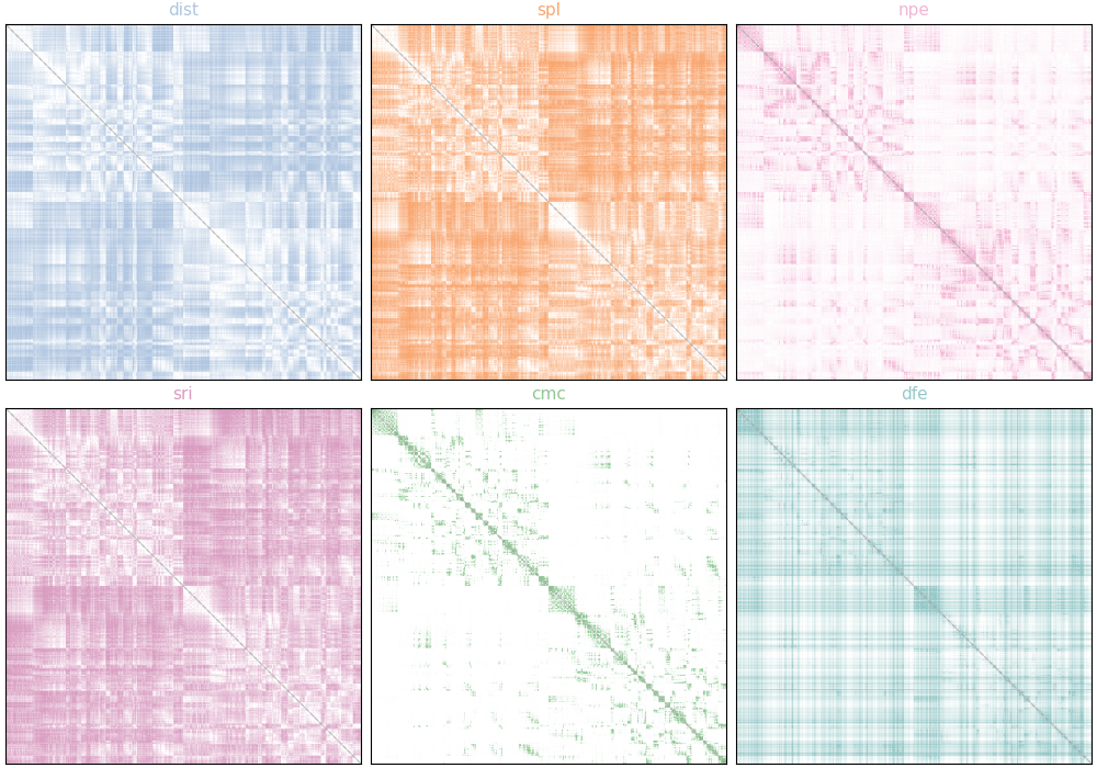
Now compute structural communication matrices using the same derivation strategy as the original analysis:

1. Convert connection weights to lengths: sc_neglog = -log(sc / (max(sc) + 1))

2. Compute shortest-path length from those lengths

3. Compute navigation path efficiency from Euclidean-guided routing

4. Compute search information, communicability, and diffusion efficiency

We then symmetrize asymmetric measures by averaging with their transpose.

from scipy.stats import zscore
from sklearn.linear_model import LinearRegression

from netneurotools.metrics import (
    communicability_wei,
    distance_wei_floyd,
    navigation_wu,
    search_information,
    mean_first_passage_time
)

# Load parcel centroids for Euclidean distance
coor = np.loadtxt(
    dataset_root / "data" / "schaefer" / "Schaefer_400_centres.txt",
    dtype=str,
)[:, 1:].astype(float)
dist_mat = scipy_cdist(coor, coor)

# Weight-to-length remapping used in the reference workflow
sc_neglog = -1.0 * np.log(SC / (np.max(SC) + 1.0))

# Shortest path length and shortest path efficiency
spl_mat, _ = distance_wei_floyd(sc_neglog)

# Navigation efficiency
_, _, npl_asym, _, nav_paths = navigation_wu(dist_mat, SC)
npe_asym = np.zeros_like(npl_asym)
finite = np.isfinite(npl_asym) & (npl_asym > 0)
npe_asym[finite] = 1.0 / npl_asym[finite]
npe_mat = (npe_asym + npe_asym.T) / 2.0

# Search information
sri_asym = search_information(SC, sc_neglog)
sri_asym = np.nan_to_num(sri_asym, nan=0.0, posinf=0.0, neginf=0.0)
sri_mat = (sri_asym + sri_asym.T) / 2.0

# Communicability
cmc_mat = communicability_wei(SC)

# Diffusion efficiency from mean first passage time
mfpt_asym = mean_first_passage_time(SC)
dfe_asym = np.zeros_like(mfpt_asym)
finite = np.isfinite(mfpt_asym) & (mfpt_asym > 0)
dfe_asym[finite] = 1.0 / mfpt_asym[finite]
dfe_mat = (dfe_asym + dfe_asym.T) / 2.0

comm_mats = [dist_mat, spl_mat, npe_mat, sri_mat, cmc_mat, dfe_mat]
comm_names = ["dist", "spl", "npe", "sri", "cmc", "dfe"]
comm_colors = ["#afc5e0", "#f9a771", "#f2b5d4", "#d99dc1", "#90c794", "#96c8c8"]

print(f"Computed {len(comm_mats)} communication matrices")

/home/runner/work/netneurotools/netneurotools/examples/plot_coupling.py:187: RuntimeWarning: divide by zero encountered in log
  sc_neglog = -1.0 * np.log(SC / (np.max(SC) + 1.0))
Computed 6 communication matrices

Visualize the communication matrices. Each uses a mode-specific gradient colormap (clipped at the 2.5th and 97.5th percentile for display).

def make_comm_cmap(hex_color):
    """Create a white-to-color gradient colormap for one communication metric."""
    rgb = to_rgb(hex_color)
    vals = np.ones((256, 4))
    vals[:, 0] = np.linspace(1.0, rgb[0], 256)
    vals[:, 1] = np.linspace(1.0, rgb[1], 256)
    vals[:, 2] = np.linspace(1.0, rgb[2], 256)
    return ListedColormap(vals)


fig, axes = plt.subplots(2, 3, figsize=(10, 7), constrained_layout=True)
axes = axes.ravel()

for i, (A, name, color) in enumerate(zip(comm_mats, comm_names, comm_colors)):
    ax = axes[i]
    A_plot = A.copy()
    np.fill_diagonal(A_plot, np.nan)
    ax.imshow(A_plot, cmap=make_comm_cmap(color),
              vmin=np.nanpercentile(A_plot, 2.5),
              vmax=np.nanpercentile(A_plot, 97.5))
    ax.set_title(name, fontsize=11, color=color)
    ax.set_xticks([])
    ax.set_yticks([])

Compute global structure-function coupling. Following the global model in Liu et al. (2023), we vectorize the upper triangle of each connectivity matrix and regress it onto the corresponding communication predictors.

nnode = SC.shape[0]
iu = np.triu_indices(nnode, k=1)
X_zs = zscore(
    np.column_stack([
        dist_mat[iu],
        spl_mat[iu],
        npe_mat[iu],
        sri_mat[iu],
        cmc_mat[iu],
        dfe_mat[iu],
    ]),
    ddof=1,
)

freq_labels = ["BOLD", *meg_bands]
fc_mats = [fc_cons, *list(meg_fc)]
sc_cplg_rsq_global = []

for _label, curr_mat in zip(freq_labels, fc_mats):
    reg = LinearRegression(fit_intercept=True, n_jobs=-1)
    y = curr_mat[iu]
    reg.fit(X_zs, y)
    yhat = reg.predict(X_zs)

    ss_res = np.sum((y - yhat) ** 2)
    ss_tot = np.sum((y - np.mean(y)) ** 2)
    r_squared = 1.0 - (float(ss_res) / ss_tot)
    adjusted_r_squared = 1.0 - (1.0 - r_squared) * (
        (len(y) - 1.0) / (len(y) - X_zs.shape[1] - 1.0)
    )
    sc_cplg_rsq_global.append(adjusted_r_squared)

sc_cplg_rsq_global = np.asarray(sc_cplg_rsq_global)

print("Global coupling analysis complete.")
for label, r2 in zip(freq_labels, sc_cplg_rsq_global):
    print(f"  {label}: adjusted R^2 = {r2:.3f}")

Global coupling analysis complete.
  BOLD: adjusted R^2 = 0.107
  delta: adjusted R^2 = 0.352
  theta: adjusted R^2 = 0.425
  alpha: adjusted R^2 = 0.314
  beta: adjusted R^2 = 0.490
  lgamma: adjusted R^2 = 0.091
  hgamma: adjusted R^2 = 0.026

Compute global dominance analysis for the same predictors and response matrices. This complements the adjusted R^2 summary by decomposing the global model into predictor-wise contributions.

from netneurotools.stats import get_dominance_stats

dom_global_list = []
for curr_mat in fc_mats:
    y = curr_mat[iu]
    model_metrics, model_r_sq = get_dominance_stats(X_zs, y, n_jobs=-1)
    dom_global_list.append((model_metrics, model_r_sq))

dom_global_total = np.array([d[0]["total_dominance"] for d in dom_global_list])
dom_global_total_ratio = dom_global_total / np.sum(
    dom_global_total, axis=1, keepdims=True
)

Display the global coupling profile across BOLD and MEG frequency bands, with stacked dominance ratios showing the relative contribution of each communication predictor.

fig, ax = plt.subplots(figsize=(10, 7))
x = np.arange(len(freq_labels))
bottom = np.zeros(len(freq_labels))

for comm_idx, comm_name in enumerate(comm_names):
    ax.bar(
        x,
        dom_global_total_ratio[:, comm_idx],
        width=0.6,
        bottom=bottom,
        label=comm_name,
        color=comm_colors[comm_idx],
        alpha=0.8,
    )
    bottom += dom_global_total_ratio[:, comm_idx]

ax.legend(frameon=False)
ax.plot(x, sc_cplg_rsq_global, lw=5, color="white")
ax.plot(x, sc_cplg_rsq_global, lw=3, color="tab:red")
ax.set_xticks(x)
ax.set_xticklabels(freq_labels, rotation=45, ha="right")
ax.set_ylim(0, max(1.0, np.max(sc_cplg_rsq_global) * 1.4))
ax.set_title("Global structure–function coupling")
plt.tight_layout()

The line summarizes global coupling (adjusted R^2) across haemodynamic and electrophysiological functional connectivity and matches the global model in Liu et al. (2023). The stacked bars provide a complementary decomposition of predictor contributions for the same global model.

A practical limitation is that the communication model is only as good as the upstream SC estimation and parcel correspondence; those preprocessing choices are intentionally outside the scope of this gallery example.