Network assortativity and distance-preserving surrogates

This example demonstrates how to calculate network assortativity and generate distance-preserving surrogate connectomes for null hypothesis testing. We’ll use structural connectivity data and myelin maps from Bazinet et al. (2023) to explore how brain network topology relates to spatial patterns of cortical features:

First, let’s fetch the structural connectivity and myelin data from Bazinet et al. (2023). This dataset contains a 400-parcel structural connectome with a corresponding distance matrix specifying the distance between parcel centroids. It also contains a T1w/T2w myelin map:

import numpy as np
import pickle
from netneurotools.datasets import fetch_bazinet_assortativity

bazinet_path = fetch_bazinet_assortativity()

with open(f'{bazinet_path}/data/human_SC_s400.pickle', 'rb') as file:
    human_data = pickle.load(file)

SC = human_data['adj']
dist = human_data['dist']
myelin = human_data['t1t2']

print(f'Structural connectivity shape: {SC.shape}')
print(f'Distance matrix shape: {dist.shape}')
print(f'Myelin data shape: {myelin.shape}')

Please cite the following papers if you are using this function:
  [primary]:
    Vincent Bazinet, Justine Y Hansen, Reinder Vos de Wael, Boris C Bernhardt, Martijn P van den Heuvel, and Bratislav Misic. Assortative mixing in micro-architecturally annotated brain connectomes. Nature Communications, 14(1):2850, 2023.
[fetch_single_file] Downloading data from
https://github.com/netneurolab/bazinet_assortativity/archive/baab96d173b8c5a2656
67a4259cf228713dabcc7.tar.gz ...
[fetch_single_file] Downloaded 13893632 of ? bytes.
[fetch_single_file] Downloaded 27525120 of ? bytes.
[fetch_single_file] Downloaded 41418752 of ? bytes.
[fetch_single_file] Downloaded 55320576 of ? bytes.
[fetch_single_file] Downloaded 59252736 of ? bytes.
[fetch_single_file] Downloaded 63184896 of ? bytes.
[fetch_single_file] Downloaded 67117056 of ? bytes.
[fetch_single_file] Downloaded 74981376 of ? bytes.
[fetch_single_file] Downloaded 94633984 of ? bytes.
[fetch_single_file] Downloaded 105906176 of ? bytes.
[fetch_single_file] Downloaded 108797952 of ? bytes.
[fetch_single_file] Downloaded 111943680 of ? bytes.
[fetch_single_file] Downloaded 115089408 of ? bytes.
[fetch_single_file] Downloaded 120635392 of ? bytes.
[fetch_single_file] Downloaded 133701632 of ? bytes.
[fetch_single_file] Downloaded 136585216 of ? bytes.
[fetch_single_file] Downloaded 139460608 of ? bytes.
[fetch_single_file] Downloaded 143138816 of ? bytes.
[fetch_single_file] Downloaded 148111360 of ? bytes.
[fetch_single_file] Downloaded 151003136 of ? bytes.
[fetch_single_file] Downloaded 155975680 of ? bytes.
[fetch_single_file] Downloaded 159391744 of ? bytes.
[fetch_single_file] Downloaded 166199296 of ? bytes.
[fetch_single_file] Downloaded 169082880 of ? bytes.
[fetch_single_file] Downloaded 171974656 of ? bytes.
[fetch_single_file] Downloaded 175120384 of ? bytes.
[fetch_single_file] Downloaded 178257920 of ? bytes.
[fetch_single_file] Downloaded 195035136 of ? bytes.
[fetch_single_file] Downloaded 204480512 of ? bytes.
[fetch_single_file] Downloaded 207355904 of ? bytes.
[fetch_single_file] Downloaded 210239488 of ? bytes.
[fetch_single_file] Downloaded 213655552 of ? bytes.
[fetch_single_file] Downloaded 217849856 of ? bytes.
[fetch_single_file] Downloaded 220733440 of ? bytes.
[fetch_single_file] Downloaded 227549184 of ? bytes.
[fetch_single_file] Downloaded 230432768 of ? bytes.
[fetch_single_file] Downloaded 233422848 of ? bytes.
[fetch_single_file] Downloaded 236199936 of ? bytes.
[fetch_single_file] Downloaded 239345664 of ? bytes.
[fetch_single_file] Downloaded 243802112 of ? bytes.
[fetch_single_file] Downloaded 247734272 of ? bytes.
[fetch_single_file] Downloaded 273424384 of ? bytes.
[fetch_single_file] Downloaded 298852352 of ? bytes.
[fetch_single_file] Downloaded 320348160 of ? bytes.
[fetch_single_file] Downloaded 340795392 of ? bytes.
[fetch_single_file] Downloaded 360726528 of ? bytes.
[fetch_single_file] Downloaded 381689856 of ? bytes.
[fetch_single_file] Downloaded 402653184 of ? bytes.
[fetch_single_file] Downloaded 420487168 of ? bytes.
[fetch_single_file] Downloaded 441712640 of ? bytes.
[fetch_single_file] Downloaded 461643776 of ? bytes.
[fetch_single_file] Downloaded 483196928 of ? bytes.
[fetch_single_file] Downloaded 502538240 of ? bytes.
[fetch_single_file] Downloaded 523771904 of ? bytes.
[fetch_single_file] Downloaded 545529856 of ? bytes.
[fetch_single_file] Downloaded 564133888 of ? bytes.
[fetch_single_file] Downloaded 586948608 of ? bytes.
[fetch_single_file]  ...done. (60 seconds, 1 min)

Downloaded ds-bazinet_assortativity to /home/runner/nnt-data
/home/runner/work/netneurotools/netneurotools/examples/plot_assortativity.py:34: DeprecationWarning: numpy.core.numeric is deprecated and has been renamed to numpy._core.numeric. The numpy._core namespace contains private NumPy internals and its use is discouraged, as NumPy internals can change without warning in any release. In practice, most real-world usage of numpy.core is to access functionality in the public NumPy API. If that is the case, use the public NumPy API. If not, you are using NumPy internals. If you would still like to access an internal attribute, use numpy._core.numeric._frombuffer.
  human_data = pickle.load(file)
Structural connectivity shape: (400, 400)
Distance matrix shape: (400, 400)
Myelin data shape: (400,)

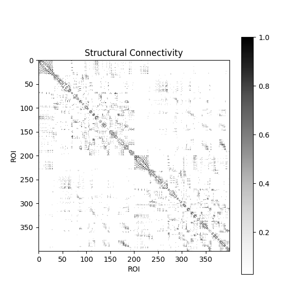
Let’s visualize the structural connectivity matrix. This shows the weighted connections between all pairs of brain regions:

import matplotlib.pyplot as plt

fig, ax = plt.subplots(figsize=(6, 6))
im = ax.imshow(SC, cmap='Greys', vmin=SC[SC > 0].min(), vmax=SC.max())
ax.set(xlabel='ROI', ylabel='ROI', title='Structural Connectivity')
fig.colorbar(im, ax=ax)

<matplotlib.colorbar.Colorbar object at 0x7ff8c4ec3e30>

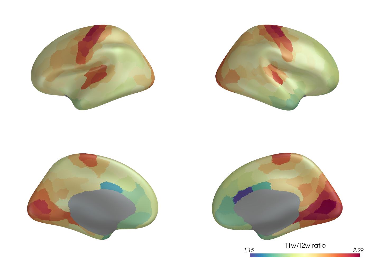
Let’s visualize the parcellated myelin data on the cortical surface. The structural connectivity and myelin data have been parcellated with the Schaefer (400 nodes) parcellation.

from netneurotools.plotting import pv_plot_parcellated_data

# This is necessary for headless rendering when building the sphinx gallery.
# If you are running this code locally, you might not need this line.
import os
os.environ["VTK_DEFAULT_OPENGL_WINDOW"] = "vtkOSOpenGLRenderWindow"

pv_plot_parcellated_data(myelin,
                         'schaefer400x7',
                         cmap='Spectral_r',
                         clim=[np.min(myelin), np.max(myelin)],
                         cbar_title='T1w/T2w ratio',
                         lighting_style='plastic',
                         jupyter_backend="static")

Please cite the following papers if you are using this function:
  [primary]:
    Alexander Schaefer, Ru Kong, Evan M Gordon, Timothy O Laumann, Xi-Nian Zuo, Avram J Holmes, Simon B Eickhoff, and BT Thomas Yeo. Local-global parcellation of the human cerebral cortex from intrinsic functional connectivity mri. Cerebral cortex, 28(9):3095–3114, 2018.
[fetch_single_file] Downloading data from
https://files.osf.io/v1/resources/udpv8/providers/osfstorage/673273c54b79ea9a506
2f4b3 ...
[fetch_single_file]  ...done. (1 seconds, 0 min)

Downloaded atl-schaefer2018 to /home/runner/nnt-data
<PIL.Image.Image image mode=RGB size=1400x1000 at 0x7FF8B6B0DCA0>

<pyvista.plotting.plotter.Plotter object at 0x7ff8cee466f0>

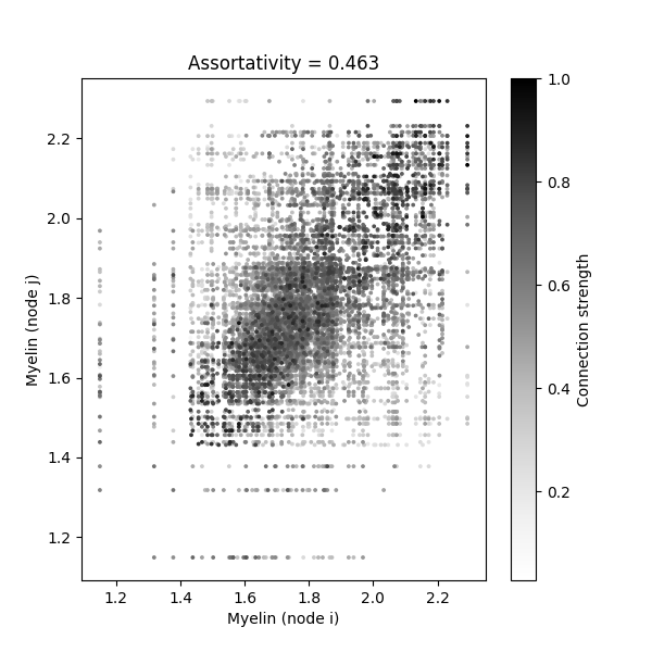
Network assortativity measures the tendency for nodes with similar features to be connected. Let’s calculate the assortativity of the myelin distribution with respect to the structural connectivity network:

from netneurotools.metrics import assortativity_und

assort = assortativity_und(myelin, SC, use_numba=False)
print(f'Network assortativity: {assort:.3f}')

Network assortativity: 0.463

We can visualize this by creating a scatterplot showing the myelin values of connected node pairs, with point colors indicating connection strength:

SC_E = SC > 0
Xi = np.repeat(myelin[np.newaxis, :], 400, axis=0)
Xj = np.repeat(myelin[:, np.newaxis], 400, axis=1)
sort_ids = np.argsort(SC[SC_E])

fig, ax = plt.subplots(figsize=(6, 6))
scatter = ax.scatter(
    Xi[SC_E][sort_ids],
    Xj[SC_E][sort_ids],
    c=SC[SC_E][sort_ids],
    cmap='Greys',
    s=3,
    rasterized=True
)
ax.set(xlabel='Myelin (node i)', ylabel='Myelin (node j)')
ax.set_title(f'Assortativity = {assort:.3f}')
fig.colorbar(scatter, ax=ax, label='Connection strength')

<matplotlib.colorbar.Colorbar object at 0x7ff8b7869790>

To test whether this assortativity is significant, we need null models that preserve key topological properties. We’ll generate distance-preserving surrogate networks that maintain the degree distribution and spatial embedding of connections. For this, we need the empirical structural connectome and a matrix specifying the distance between each parcel.

Note: Generating many surrogates can be time-consuming. For this example, we’ll create just a few surrogates:

from netneurotools.networks import match_length_degree_distribution

n_surrogates = 10
surr_all = np.zeros((n_surrogates, 400, 400))

for i in range(n_surrogates):
    surr_all[i] = match_length_degree_distribution(SC, dist)[1]

print(f'Generated {n_surrogates} surrogate networks')

Generated 10 surrogate networks

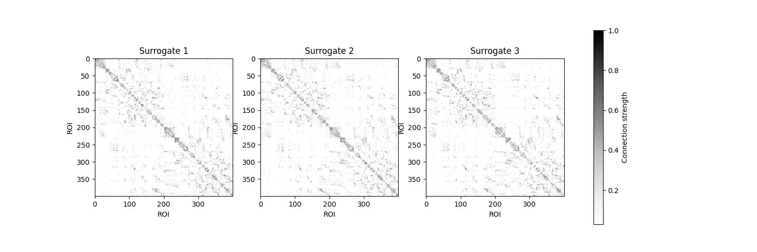
Let’s visualize a few of these surrogate connectomes to see how they compare to the empirical network:

fig, axes = plt.subplots(1, 3, figsize=(15, 5))
for i, ax in enumerate(axes):
    im = ax.imshow(
        surr_all[i],
        cmap='Greys',
        vmin=surr_all[i][surr_all[i] > 0].min(),
        vmax=surr_all[i].max()
    )
    ax.set_title(f'Surrogate {i + 1}')
    ax.set(xlabel='ROI', ylabel='ROI')
fig.colorbar(im, ax=axes.ravel().tolist(), label='Connection strength')

<matplotlib.colorbar.Colorbar object at 0x7ff8b78476e0>

Now we’ll calculate the assortativity for each surrogate network to create a null distribution:

assort_surr = np.zeros(n_surrogates)
for i in range(n_surrogates):
    assort_surr[i] = assortativity_und(myelin, surr_all[i])

print(f'Mean surrogate assortativity: {np.mean(assort_surr):.3f}')
print(f'Std surrogate assortativity: {np.std(assort_surr):.3f}')

Mean surrogate assortativity: 0.400
Std surrogate assortativity: 0.006

Finally, we can compare the empirical assortativity to the null distribution using a boxplot. This visualization shows whether the observed assortativity is significantly different from what we’d expect by chance:

fig, ax = plt.subplots(figsize=(4, 6))

flierprops = dict(
    marker='+',
    markerfacecolor='lightgray',
    markeredgecolor='lightgray'
)

bplot = ax.boxplot(
    assort_surr,
    widths=0.3,
    patch_artist=True,
    showfliers=True,
    showcaps=False,
    flierprops=flierprops
)

for box in bplot['boxes']:
    box.set(facecolor='lightgray', edgecolor='black')
for median in bplot['medians']:
    median.set(color='black', linewidth=2)

ax.scatter(1, assort, color='red', s=100, zorder=3, label='Empirical')
ax.set_xticks([1])
ax.set_xticklabels(['Surrogates'])
ax.set_ylabel('Assortativity')
ax.set_title('Empirical vs. Null Distribution')
ax.legend()
ax.set_xlim(0.7, 1.3)

plt.tight_layout()

The red dot shows the empirical assortativity, while the boxplot shows the distribution of assortativity values from the distance-preserving surrogate networks. If the empirical value falls outside the null distribution, this suggests that the observed pattern of myelin assortativity is not explained by the spatial constraints and topology of the connectome alone.

The limitation is equally important: geometry-aware nulls still depend on the quality of the upstream surface / centroid information, and generating large surrogate ensembles can be computationally expensive.