Are brain modules consistent across connectivity modes?

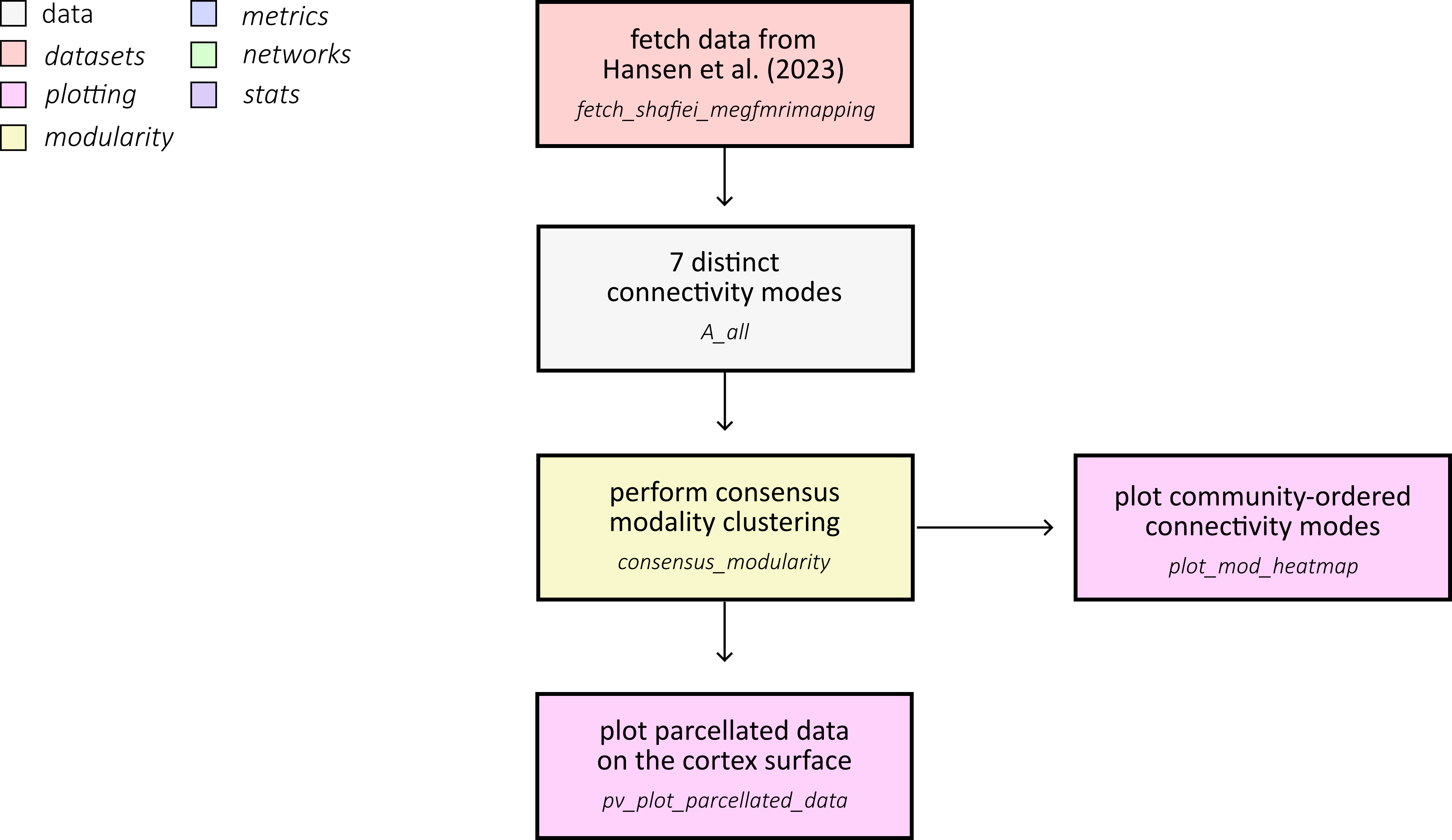
This example reproduces the core workflow used to compare mesoscale community structure across multiple cortical connectivity modes from Hansen et al. (2023). We load seven connectivity matrices, inspect how the number of communities changes with resolution, and summarize mode-specific community assignments:

First, fetch the multimodal connectivity dataset from Hansen et al. (2023) and load all Schaefer-400 connectivity matrices used in the comparison.

from pathlib import Path

import matplotlib.pyplot as plt
import numpy as np
from matplotlib.colors import ListedColormap, to_rgb

from netneurotools.datasets import fetch_hansen_manynetworks

dataset_root = Path(fetch_hansen_manynetworks())
data_dir = dataset_root / "data" / "Schaefer400"

matrix_files = [
    "gene_coexpression.npy",
    "receptor_similarity.npy",
    "laminar_similarity.npy",
    "metabolic_connectivity.npy",
    "haemodynamic_connectivity.npy",
    "electrophysiological_connectivity.npy",
    "temporal_similarity.npy",
]
mode_labels = [
    "gene",
    "receptor",
    "laminar",
    "metabolic",
    "haemodynamic",
    "electrophysiological",
    "temporal",
]
mode_abbrev = ["gc", "rs", "ls", "mc", "hc", "ec", "ts"]

Please cite the following papers if you are using this function:
  [primary]:
    Justine Y Hansen, Golia Shafiei, Katharina Voigt, Emma X Liang, Sylvia ML Cox, Marco Leyton, Sharna D Jamadar, and Bratislav Misic. Integrating multimodal and multiscale connectivity blueprints of the human cerebral cortex in health and disease. PLoS biology, 21(9):e3002314, 2023.
  [gene]:
    Hawrylycz, M. J., Lein, E. S., Guillozet-Bongaarts, A. L., Shen, E. H., Ng, L., Miller, J. A., ... & Jones, A. R. (2012). An anatomically comprehensive atlas of the adult human brain transcriptome. Nature, 489(7416), 391-399.
  [receptor]:
    Hansen, J. Y., Shafiei, G., Markello, R. D., Smart, K., Cox, S. M., Nørgaard, M., ... & Misic, B. (2022). Mapping neurotransmitter systems to the structural and functional organization of the human neocortex. Nature neuroscience, 25(11), 1569-1581.
  [larminar]:
    Paquola, C., Vos De Wael, R., Wagstyl, K., Bethlehem, R. A., Hong, S. J., Seidlitz, J., ... & Bernhardt, B. C. (2019). Microstructural and functional gradients are increasingly dissociated in transmodal cortices. PLoS biology, 17(5), e3000284.
  [metabolic]:
    Jamadar, S. D., Ward, P. G., Close, T. G., Fornito, A., Premaratne, M., O’Brien, K., ... & Egan, G. F. (2020). Simultaneous BOLD-fMRI and constant infusion FDG-PET data of the resting human brain. Scientific data, 7(1), 363.
  [haemodynamic]:
    Van Essen, D. C., Smith, S. M., Barch, D. M., Behrens, T. E., Yacoub, E., Ugurbil, K., & Wu-Minn HCP Consortium. (2013). The WU-Minn human connectome project: an overview. Neuroimage, 80, 62-79.
  [electrophysiological]:
    Shafiei, G., Baillet, S., & Misic, B. (2022). Human electromagnetic and haemodynamic networks systematically converge in unimodal cortex and diverge in transmodal cortex. PLoS biology, 20(8), e3001735.
  [temporal]:
    Shafiei, G., Markello, R. D., Vos de Wael, R., Bernhardt, B. C., Fulcher, B. D., & Misic, B. (2020). Topographic gradients of intrinsic dynamics across neocortex. elife, 9, e62116.
  [cognitive]:

[fetch_single_file] Downloading data from
https://github.com/netneurolab/hansen_many_networks/archive/72b4b3dc2983bf9baf00
00926a610ead73b91b1d.tar.gz ...
[fetch_single_file] Downloaded 18096128 of ? bytes.
[fetch_single_file] Downloaded 21766144 of ? bytes.
[fetch_single_file] Downloaded 38805504 of ? bytes.
[fetch_single_file] Downloaded 50601984 of ? bytes.
[fetch_single_file] Downloaded 54788096 of ? bytes.
[fetch_single_file]  ...done. (6 seconds, 0 min)

Downloaded ds-hansen_manynetworks to /home/runner/nnt-data

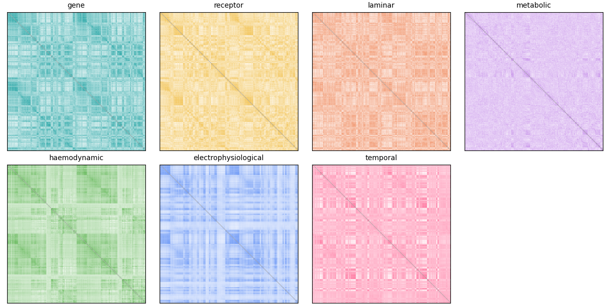
The seven connectivity modes span molecular, microstructural, metabolic, haemodynamic, electrophysiological, and temporal domains:

1. gene coexpression: transcriptional similarity from AHBA (Hawrylycz et al. (2012)).

2. receptor similarity: correspondence in neurotransmitter receptor/ transporter profiles (Hansen et al. (2022)).

3. laminar similarity: similarity of cortical microstructure profiles derived from BigBrain (Paquola et al. (2019); Amunts et al. (2013)).

4. metabolic connectivity: coupling of dynamic FDG-fPET signals (Jamadar et al. (2021); Jamadar et al. (2020)).

5. haemodynamic connectivity: resting-state BOLD fMRI coupling from HCP (Van Essen et al. (2013)).

6. electrophysiological connectivity: MEG-derived connectivity summary across canonical frequency bands (Van Essen et al. (2013); Shafiei et al. (2022)).

7. temporal profile similarity: similarity of rich BOLD time-series features (Shafiei et al. (2020); Fulcher et al. (2013); Fulcher and Jones (2017)).

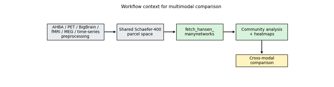
In the source dataset, all networks are represented at Schaefer-400 and harmonized for cross-modal comparison (Schaefer et al. (2018)).

A_all = []
for file_name in matrix_files:
    A = np.load(data_dir / file_name)
    np.fill_diagonal(A, np.nan)
    A_all.append(A)

print(f"Loaded {len(A_all)} connectivity modes from: {data_dir}")

Loaded 7 connectivity modes from: /home/runner/nnt-data/ds-hansen_manynetworks/data/Schaefer400

We can start by plotting each matrix:

base_colors = [
    "#2ca8a8",  # gene
    "#f2c14e",  # receptor
    "#f08a5d",  # laminar
    "#c792ea",  # metabolic
    "#73bf69",  # haemodynamic
    "#7aa2f7",  # electrophysiological
    "#ff7aa2",  # temporal
]


def make_mode_cmap(hex_color):
    """Create a white-to-color gradient colormap for one connectivity mode."""
    rgb = to_rgb(hex_color)
    vals = np.ones((256, 4))
    vals[:, 0] = np.linspace(1.0, rgb[0], 256)
    vals[:, 1] = np.linspace(1.0, rgb[1], 256)
    vals[:, 2] = np.linspace(1.0, rgb[2], 256)
    return ListedColormap(vals)


fig, axes = plt.subplots(2, 4, figsize=(12, 6), constrained_layout=True)
axes = axes.ravel()

for i, (A, label) in enumerate(zip(A_all, mode_labels)):
    ax = axes[i]
    vmax = np.nanmean(A) + 3 * np.nanstd(A)
    vmin = np.nanmean(A) - 3 * np.nanstd(A)
    ax.imshow(A, cmap=make_mode_cmap(base_colors[i]), vmin=vmin, vmax=vmax)
    ax.set_title(label, fontsize=10)
    ax.set_xticks([])
    ax.set_yticks([])

# Hide the final empty panel in the 2x4 layout.
axes[-1].axis("off")

(np.float64(0.0), np.float64(1.0), np.float64(0.0), np.float64(1.0))

Next, we’ll run community detection across a range of resolution parameters. The workflow below applies consensus modularity clustering with negative asymmetry null model across 60 resolution parameters (gamma from 0.1 to 6.0). We leave it in comments to avoid running a long analysis in the example, but you can run it locally if you have the resources. The results are saved to disk and loaded in the next section for visualization.

# from netneurotools.modularity import consensus_modularity
# from joblib import Parallel, delayed

# def community_detection(A, gamma_range):
#     """Run consensus modularity clustering for a range of gamma values."""
#     nnodes = len(A)
#     ngamma = len(gamma_range)
#     consensus = np.zeros((nnodes, ngamma))
#     qall = []
#     zrand = []
#     for i, g in enumerate(gamma_range):
#         consensus[:, i], q, z = consensus_modularity(
#             A, g, B='negative_asym'
#         )
#         qall.append(q)
#         zrand.append(z)
#     return consensus, qall, zrand

# # Load and preprocess connectivity matrices
# networks = {
#     "gc": np.load(data_dir / "gene_coexpression.npy"),
#     "rs": np.load(data_dir / "receptor_similarity.npy"),
#     "ls": np.load(data_dir / "laminar_similarity.npy"),
#     "mc": np.load(data_dir / "metabolic_connectivity.npy"),
#     "hc": np.load(data_dir / "haemodynamic_connectivity.npy"),
#     "ec": np.load(data_dir / "electrophysiological_connectivity.npy"),
#     "ts": np.load(data_dir / "temporal_similarity.npy"),
# }
# # Fisher's z-transform and zero diagonal
# for network in networks.keys():
#     networks[network] = np.arctanh(networks[network])
#     networks[network][np.eye(len(networks[network])).astype(bool)] = 0

# # Run community detection in parallel
# gamma_range = [x / 10.0 for x in range(1, 61, 1)]
# output = Parallel(n_jobs=36)(
#     delayed(community_detection)(networks[network], gamma_range)
#     for network in networks.keys()
# )

# # Save results
# results_dir = dataset_root / "results" / "community_detection_Schaefer400"
# results_dir.mkdir(parents=True, exist_ok=True)
# for network_idx, network_name in enumerate(networks.keys()):
#     np.save(
#         results_dir / f"community_assignments_{network_name}.npy",
#         output[network_idx][0]
#     )
#     np.save(
#         results_dir / f"community_qall_{network_name}.npy",
#         np.array(output[network_idx][1])
#     )
#     np.save(
#         results_dir / f"community_zrand_{network_name}.npy",
#         np.array(output[network_idx][2])
#     )

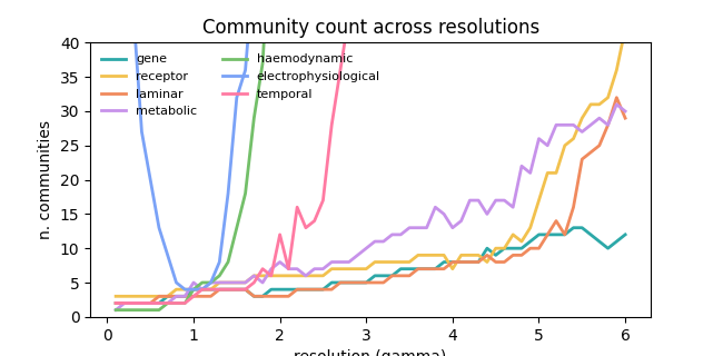
To save time, we load precomputed community assignments across a range of resolution parameters and inspect the number of detected communities per mode.

results_dir = dataset_root / "results" / "community_detection_Schaefer400"
y_grid = np.linspace(0.1, 6.0, 60)

ci_all = []
for abb in mode_abbrev:
    ci_path = results_dir / f"community_assignments_{abb}.npy"
    ci_all.append(np.load(ci_path))

fig, ax = plt.subplots(figsize=(6.5, 3.2))
for i, (ci, label) in enumerate(zip(ci_all, mode_labels)):
    n_communities = np.max(ci, axis=0)
    ax.plot(y_grid, n_communities, color=base_colors[i], linewidth=2, label=label)

ax.set(
    xlabel="resolution (gamma)",
    ylabel="n. communities",
    ylim=(0, 40),
    title="Community count across resolutions",
)
ax.legend(ncol=2, frameon=False, fontsize=8)

<matplotlib.legend.Legend object at 0x7f94582ec590>

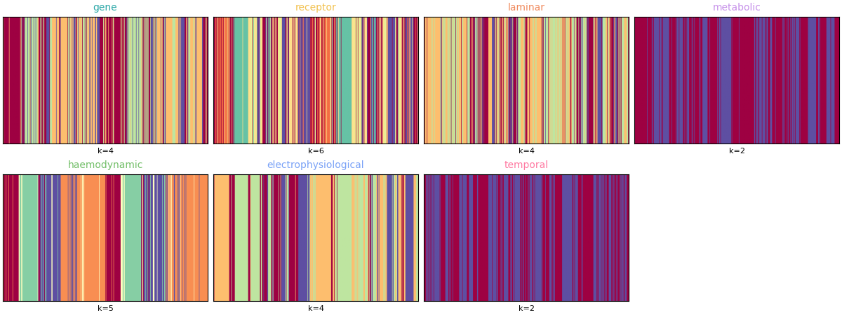
Finally, summarize one representative partition per mode (chosen from the same resolution indices as the original analysis) using community assignment matrices instead of brain-surface renderings.

y_best = [19, 19, 24, 4, 11, 9, 6]

fig, axes = plt.subplots(2, 4, figsize=(12, 4.5), constrained_layout=True)
axes = axes.ravel()

for i, (ci, label) in enumerate(zip(ci_all, mode_labels)):
    ax = axes[i]
    ci_best = ci[:, y_best[i]]
    # Plot as a 1 x N matrix for quick visual comparison across modes.
    ax.imshow(ci_best[np.newaxis, :], aspect="auto", cmap="Spectral")
    ax.set_title(label, fontsize=10, color=base_colors[i])
    ax.set_xticks([])
    ax.set_yticks([])
    ax.set_xlabel(f"k={int(np.max(ci_best))}", fontsize=8)

axes[-1].axis("off")

(np.float64(0.0), np.float64(1.0), np.float64(0.0), np.float64(1.0))

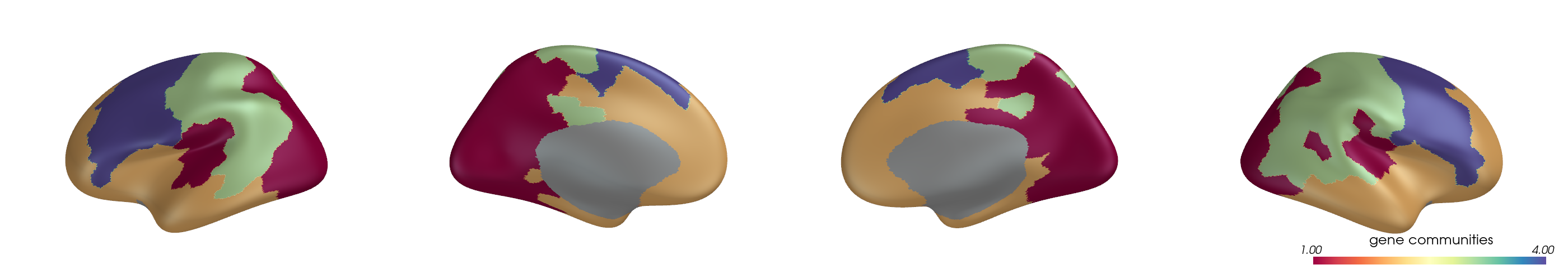
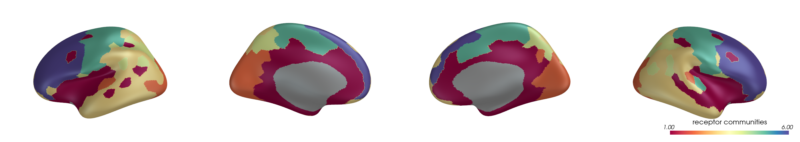
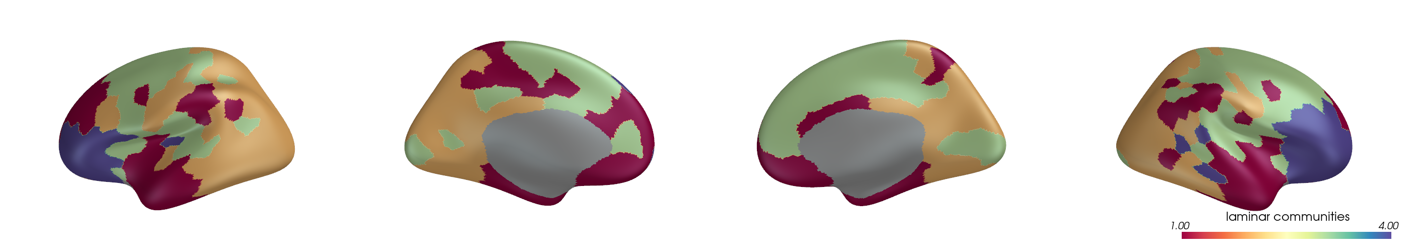
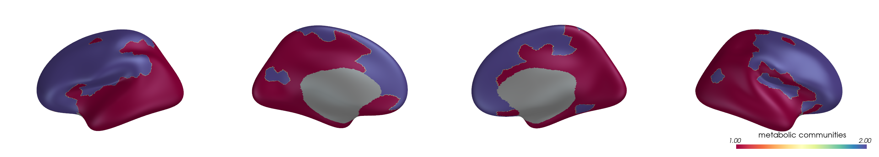
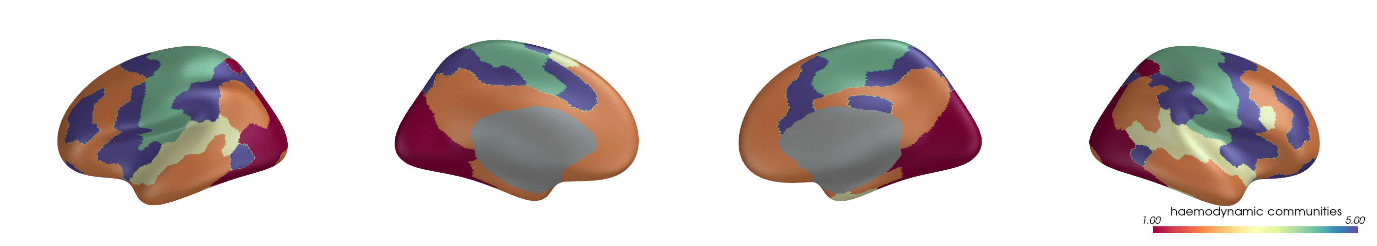
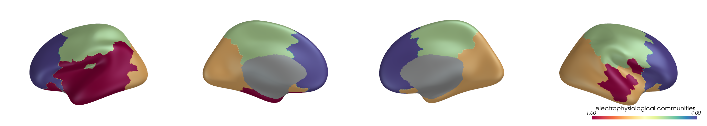
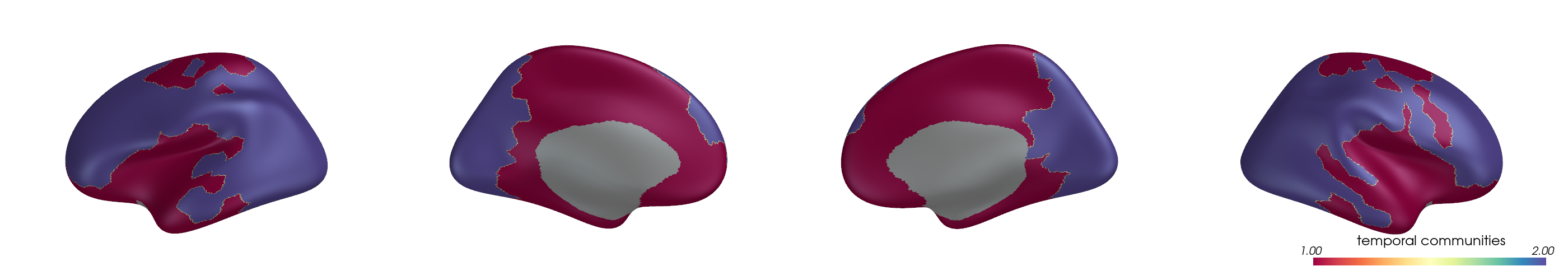
You can project parcel-wise community assignments to fsaverage vertices and render them on an inflated surface.

from netneurotools.plotting import pv_plot_parcellated_data

# This is necessary for headless rendering when building the sphinx gallery.
# If you are running this code locally, you might not need this line.
import os
os.environ["VTK_DEFAULT_OPENGL_WINDOW"] = "vtkOSOpenGLRenderWindow"

for i, (ci, label) in enumerate(zip(ci_all, mode_labels)):
    ci_best = ci[:, y_best[i]]

    pv_plot_parcellated_data(
        ci_best,
        "schaefer400x7",
        cmap="Spectral",
        cbar_title=f"{label} communities",
        layout="row",
        lighting_style='plastic'
    )

• 
• 
• 
• 
• 
• 
• 

Please cite the following papers if you are using this function:
  [primary]:
    Alexander Schaefer, Ru Kong, Evan M Gordon, Timothy O Laumann, Xi-Nian Zuo, Avram J Holmes, Simon B Eickhoff, and BT Thomas Yeo. Local-global parcellation of the human cerebral cortex from intrinsic functional connectivity mri. Cerebral cortex, 28(9):3095–3114, 2018.
Dataset atl-schaefer2018 already exists. Skipping download.
<PIL.Image.Image image mode=RGB size=2800x500 at 0x7F9459527920>
Please cite the following papers if you are using this function:
  [primary]:
    Alexander Schaefer, Ru Kong, Evan M Gordon, Timothy O Laumann, Xi-Nian Zuo, Avram J Holmes, Simon B Eickhoff, and BT Thomas Yeo. Local-global parcellation of the human cerebral cortex from intrinsic functional connectivity mri. Cerebral cortex, 28(9):3095–3114, 2018.
Dataset atl-schaefer2018 already exists. Skipping download.
<PIL.Image.Image image mode=RGB size=2800x500 at 0x7F94840867B0>
Please cite the following papers if you are using this function:
  [primary]:
    Alexander Schaefer, Ru Kong, Evan M Gordon, Timothy O Laumann, Xi-Nian Zuo, Avram J Holmes, Simon B Eickhoff, and BT Thomas Yeo. Local-global parcellation of the human cerebral cortex from intrinsic functional connectivity mri. Cerebral cortex, 28(9):3095–3114, 2018.
Dataset atl-schaefer2018 already exists. Skipping download.
<PIL.Image.Image image mode=RGB size=2800x500 at 0x7F9486399370>
Please cite the following papers if you are using this function:
  [primary]:
    Alexander Schaefer, Ru Kong, Evan M Gordon, Timothy O Laumann, Xi-Nian Zuo, Avram J Holmes, Simon B Eickhoff, and BT Thomas Yeo. Local-global parcellation of the human cerebral cortex from intrinsic functional connectivity mri. Cerebral cortex, 28(9):3095–3114, 2018.
Dataset atl-schaefer2018 already exists. Skipping download.
<PIL.Image.Image image mode=RGB size=2800x500 at 0x7F94998698B0>
Please cite the following papers if you are using this function:
  [primary]:
    Alexander Schaefer, Ru Kong, Evan M Gordon, Timothy O Laumann, Xi-Nian Zuo, Avram J Holmes, Simon B Eickhoff, and BT Thomas Yeo. Local-global parcellation of the human cerebral cortex from intrinsic functional connectivity mri. Cerebral cortex, 28(9):3095–3114, 2018.
Dataset atl-schaefer2018 already exists. Skipping download.
<PIL.Image.Image image mode=RGB size=2800x500 at 0x7F94594C3170>
Please cite the following papers if you are using this function:
  [primary]:
    Alexander Schaefer, Ru Kong, Evan M Gordon, Timothy O Laumann, Xi-Nian Zuo, Avram J Holmes, Simon B Eickhoff, and BT Thomas Yeo. Local-global parcellation of the human cerebral cortex from intrinsic functional connectivity mri. Cerebral cortex, 28(9):3095–3114, 2018.
Dataset atl-schaefer2018 already exists. Skipping download.
<PIL.Image.Image image mode=RGB size=2800x500 at 0x7F9459423680>
Please cite the following papers if you are using this function:
  [primary]:
    Alexander Schaefer, Ru Kong, Evan M Gordon, Timothy O Laumann, Xi-Nian Zuo, Avram J Holmes, Simon B Eickhoff, and BT Thomas Yeo. Local-global parcellation of the human cerebral cortex from intrinsic functional connectivity mri. Cerebral cortex, 28(9):3095–3114, 2018.
Dataset atl-schaefer2018 already exists. Skipping download.
<PIL.Image.Image image mode=RGB size=2800x500 at 0x7F94864BB410>

Similar to the consensus-clustering example, we can also visualize each mode as a community-ordered heatmap using plot_mod_heatmap().

from netneurotools import plotting

fig, axes = plt.subplots(2, 4, figsize=(13, 7), constrained_layout=True)
axes = axes.ravel()

for i, (A, ci, label) in enumerate(zip(A_all, ci_all, mode_labels)):
    ax = axes[i]
    ci_best = ci[:, y_best[i]]
    plotting.plot_mod_heatmap(
        A,
        ci_best,
        ax=ax,
        cmap="viridis",
        cbar=False,
    )
    ax.set_title(
        f"{label} (k={int(np.max(ci_best))})",
        fontsize=10,
        color=base_colors[i],
    )

axes[-1].axis("off")

(np.float64(0.0), np.float64(1.0), np.float64(0.0), np.float64(1.0))

These panels provide a compact, modality-by-modality view of community organization: the curve plot shows how module count evolves with gamma, while the assignment matrices show differences in parcel-wise partitioning at representative resolutions.

The main limitation is deliberate: this example starts from harmonized, publication-ready matrices, so modality-specific preprocessing choices remain upstream of the workflow shown here.